

The 8-iso-PGF2α / PGF2α ratio is a newly developed approach to quantitatively distinguish the different sources of the popular biomarker of oxidative stress 8-iso-prostaglandin F2α. It is based on work by van ‘t Erve et al.[1] The tool provided on this website will allow you to analyze your own data using our approach. Please see the following references for more information and experimental results with this approach.
References:
- van ‘t Erve TJ, Lih FB, Kadiiska MB, Deterding LJ, Eling TE, Mason RP. (2015) Reinterpreting the best biomarker of oxidative stress: The 8-iso-PGF2α / PGF2α ratio distinguishes chemical from enzymatic lipid peroxidation. Free Radic Biol Med. 83:245-251 DOI: 10.1016/j.freeradbiomed.2015.03.004 [Abstract van ‘t Erve TJ, Lih FB, Kadiiska MB, Deterding LJ, Eling TE, Mason RP. (2015) Reinterpreting the best biomarker of oxidative stress: The 8-iso-PGF2α / PGF2α ratio distinguishes chemical from enzymatic lipid peroxidation. Free Radic Biol Med. 83:245-251 DOI: 10.1016/j.freeradbiomed.2015.03.004]
Download:
- Example Labels (13KB)
- 8-iso_shiny.zip (7KB)
- Example Data (15KB)
Tools for Calculations and Statistical Analysis
To facilitate adoption of the 8-iso-PGF2α / PGF2α ratio, we have created tools with detailed instruction to perform the distinguishing of the sources of 8-iso-PGF2α as well as accompanying statistical analysis in a single, user friendly, program. The program is functions as a freely downloadable module to the popular free statistical analysis program R with a custom graphical user interface. To get started, the following programs will need to have downloaded and installed the following program:
This webpage provides detailed instructions; as well as downloadable excel templates, and R files for the graphical interface. The graphical interface (8-iso_shiny.zip) should be extracted to your hard-drive prior to use.
Detailed Tutorial
9.0 - POWFIT - powder spectrum simulations
Format of the input dataset:
Before statistical analysis, your raw data needs to be formatted in a specific manner for it to be readable by the CLME program. Two separate excel files (.xlsx) need to be provided 1) the raw data, and 2) the group names. How each file is expected to look is described below.
Data
- The file should consist of 3 columns:
- Column A is for group number (this should have integers larger than 0), this column should be sorted in numerical order.
- Column B is the measured value for 8-iso-prostaglandin F2α.
- Column C is the measured value for prostaglandin F2α.
- Each row have a group number and experimental results of one experimental unit e.g. one animal, one plasma specimen, one cell extract, etc. (Table 1). Mean values for the groups should not be entered, and will be calculated by the program.
- It is important that both values for 8-iso-prostaglandin F2α and prostaglandin F2α have the same unit or else the calculation will provide meaningless results.
| Table 1: Example of CLME data file | ||
|---|---|---|
| Group | 8-iso-prostaglandin F2α | prostaglandin F2α |
| 0 | 0.07 | 1.00 |
| 0 | 0.11 | 1.64 |
| 1 | 0.04 | 0.05 |
| 1 | 0.06 | 0.07 |
| 1 | 0.02 | 0.02 |
| 3 | 0.36 | 0.77 |
| 3 | 0.28 | 0.84 |
Labels
- The file should consist of 4 columns:
- Column A is for group number (this should have integers larger than 0), this column should be sorted in numerical order.
- Column B is the description of experimental units with the group number filled in in Column A. this column will be the labels for graphical presentation.
- Column C is an integer starting with 1 and numbering down in numerical order to the last group.
- Column D represents the number of experimental units (not automatically calculated) and this should match the amount of experimental units entered in the data table (compare Table 1 to 2).
- Each represents a single group; all groups in the data table should be identified.
| Table 2: Example of CLME label file | |||
|---|---|---|---|
| Group | Name | OriGroup | N |
| 0 | Healthy rat | 1 | 2 |
| 1 | Healthy human males | 2 | 3 |
| 3 | 120 mg/kg CCI4 7h | 3 | 2 |
R and CLME
9.0 - POWFIT - powder spectrum simulations
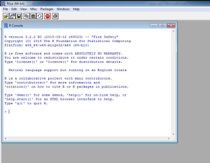
After installing R for windows on your computer open the program and you will be presented with a window similar to Figure 1.
New user only (perform once):
Download and install the following packages by typing in the following commands:
- install.packages(“CLME”)
- install.packages(“ggplot2”)
- install.packages(“multcomp”)
- Note: A pop-up might appear asking you to select a download location, please select a location near you for a fast download.
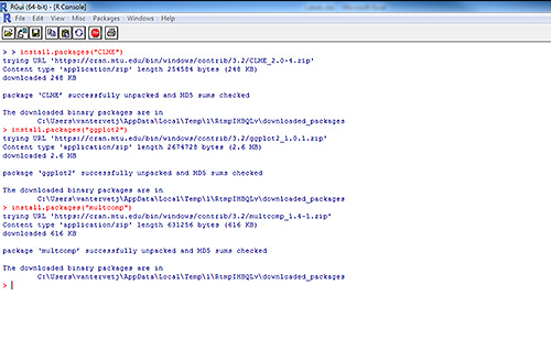
The following text will appear in your console indicating you have successfully installed the required software (Figure 2).
All users:
Load the necessary programs by typing the following commands:
- library("CLME")
- library("ggplot2")
- library("multcomp")
Under the menu “file” select the open ‘Change dir..” and browse to the folder you extracted the graphical user interface file to (8-iso_shiny.zip).
Type the following command and hit enter:
- source(shiny_iso.r")
This will start the graphical interface in your web browser and will look like Figure 3.
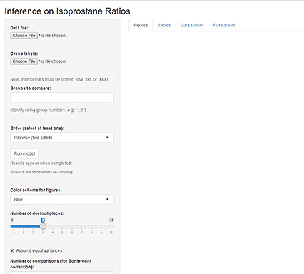
On the left side of the screen, there are multiple options:
Data file: This is where you can browse and load the data file generated previously.
Group labels: This is where you can browse and load the labels file generated previously.
Groups to compare: Enter the group numbers in numerical order which you want to compare separated by a coma.
Order: Determines how groups are compared,
- Pairwise: should be selected if the groups to be compared can both be increased or decreased from each other
- Simple: from group # A to B only an increase is expected (dose response).
- Tree: first group is control, all other groups increase from this control group.
Run model: initiated calculations and should be selected once all settings are entered.
Color scheme: changes colors in the graphs once the model is run.
Number of decimal places: changes the number of decimals reported in the mean and standard error fields of the table layout.
Assume equal variances: This will force all standard errors to be similar across all groups; can be toggled if appropriate at your discretion.
Number of comparisons: This should be equal to 1
Number of bootstrap samples: This number determines the bootstrap sample; a larger number will give more accurate results but will take longer to compute.
All other parameters should not need to be changed under normal use.
Once all files are loaded and the desired settings entered into the program, press “Run model”
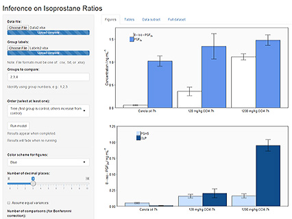
Your result will be presented in three tabs which can be selected from the top menu and consist of 3 graphs (Figures), 5 tables (Tables), and two datasets (Data subset, and Full dataset) where all computed and entered values can be viewed for quality control or troubleshooting. Figure 4 shows a typical output window.
- Note: the default unit on the graphs is ng mL-1; this can currently not be changed but also does not affect any calculation. As noted before, the entered values for 8-iso-PGF2α and PGF2α need to be in the same unit for the program to provide accurate results.
- Best practice is to generate one data file with all values and then run the model for each comparison desired.
Common Error Messages
Replacement has length zero: Group entered for comparison has no values or label associated with it.
Infinite or missing values in 'x’: Bootstrap sample is too large due to small sample size; reduce bootstrap sample number.