Overview
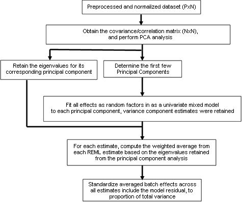
Often times "batch effects" are present in microarray data due to any number of factors, including e.g. a poor experimental design or when the gene expression data is combined from different studies with limited standardization. To estimate the variability of experimental effects including batch, a novel hybrid approach known as principal variance component analysis (PVCA) has been developed. The approach leverages the strengths of two very popular data analysis methods: first, principal component analysis (PCA) is used to efficiently reduce data dimension with maintaining the majority of the variability in the data, and variance components analysis (VCA) fits a mixed linear model using factors of interest as random effects to estimate and partition the total variability. The PVCA approach can be used as a screening tool to determine which sources of variability (biological, technical or other) are most prominent in a given microarray data set. Using the eigenvalues associated with their corresponding eigenvectors as weights, associated variations of all factors are standardized and the magnitude of each source of variability (including each batch effect) is presented as a proportion of total variance. Although PVCA is a generic approach for quantifying the corresponding proportion of variation of each effect, it can be a handy assessment for estimating batch effect before and after batch normalization.
PVCA Methods
Principal Component Analysis
Principal component analysis (PCA) is a type of dimension reduction procedure. PCA has two major features: (1) through algebraic projection, it represents the original data in a new data space with the same order; however, the axes (principal components) in the new data space are orthogonal to each other and (2) the newly formed axes are ordered in a sequentially reduced fashion in term of their weight, i.e. any given principal component captures more variability than the one that immediately follows it.
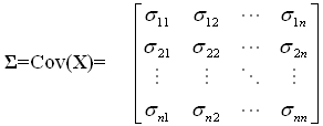
A microarray gene expression experiment researchers often deal with a data matrix (pxn), where "p" indicates total number of probes on an array and "n" represents the number of arrays applied. A random vector matrix X' =[X1, X2, …Xn] is used, where each array-associated random variable Xi has p observations. The random vector X' has the variance-covariance matrix Σ. Going through all n random variables, the variance-covariance matrix is expressed as follows:
The diagonal contains the variance measures for each random variable and off-diagonal are all pair-wise (co)variance measures. In an ideal situation (no systematic error and/or batch effect), this variance-covariance matrix contains the important biological information. Through the application of sophisticated statistical procedures, one can reveal such information by dissecting and manipulating such a matrix. Starting from our variance-covariance matrix ? of nxn, we try to find a list of n scalars (eigenvalues) λ1, λ2,...,λn satisfying the polynomial equation |?C -λC|=0, where C denotes an matrix (of eigenvector) of nxn. These scalars are also sorted in the order such that λ1 ≥ λ2 ≥...≥ λn ≥ 0. Next, for each eigenvalue λi, the corresponding eigenvector ei (nx1) can be extracted by solving ?ei= λiei. The last step is to obtain the principal components by projecting data matrix X onto corresponding eigenvector. For each eigenvalue-eigenvector pairs (λi, ei), the newly formed ith principal component is given by equation 2:
Equation 2:
PC i = Yi = e i 'X = e i1 X 1 + e i2 X 2 ... + e in Xn
In theory, eigenvalue λi represents for the corresponding variance associated to the ith principal component with the summation of all eigenvalue, Σλi, equals to the total variance of the data matrix. Also, through such a procedure to obtain eigenvalues and eigenvector pairs, the principal components are mutually orthogonal, which implies that the covariance between two principal components is zero: Cov(Yi, Yj)=0 Please refer to any good multivariate statistical methods book for details. Algebraically, the newly formed principal components are linear combination of the original random variables X1, X2,.. Xn with a constraint that the first principal component carries the highest proportion, λ1 / Σλi, of variability and the next component carries the second highest proportion, λ2 / Σλi, of variability, so on and so forth. Since the principal components are ordered according to its eigenvalues, it is sufficient to select the first x principal components (x<n) containing an amount of variation larger than a pre-defined percentage threshold (i.e. 60-90%).
Variance Component Analysis and Mixed Linear Models
Typical variation in microarray data can be regarded as random effects. The statistical model to fit an experiment design that includes both fixed effects and random effects is called a mixed model, and the variance of each random effect is called a variance component. A standard procedure for estimating variance components is described below. In a general linear model y = Xβ + e, where y denotes the vector of observations, X is the known matrix for each Xij's, β is the known fixed-effects parameter vector, and e is the unobserved vector of independent and identically distributed (iid) Gaussian random errors, Ve = σ 2 I. The general format of a mixed linear model is: y = Xβ + Zu + e, besides the same terms denoted in a fixed effect model, Z is the design matrix for random effects, u is the vector of unknown random-effect parameters, and e is the unobserved vector of iid Gaussian random errors. Here, we assume that u and e are normally distributed with:
R Script (1MB)
Given that the variance of y is V=ZGZ' + R, V can be modeled by setting up the random effects design matrix Z and by specifying the variance-covariance structure for G and R. In usual variance component models, G is a diagonal matrix with variance components on the diagonal, each replicated along the diagonal correspond to the design matrix Z. R is simply the residual variance component times the n x n identity matrix. Thus, the goal becomes finding a reasonable estimate of G and R. The method of restricted maximum likelihood (REML) is the standard procedure. In SAS, PROC MIXED is a standard tool for fitting REML estimation of variance components (see the online doc) in R it is the nlme package for fitting linear and non-linear mixed effects models.
Workflow for PVCA

References for Citing
Scherer A. Batch Effect and Experimental Noise in Microarray Studies: Sources and Solutions (2009), John Wiley & Sons
Boedigheimer MJ, Wolfinger RD, Bass MB, Bushel PR, Chou JW, Cooper M, Corton JC, Fostel J, Hester S, Lee JS, Liu F, Liu J, Qian HR, Quackenbush J, Pettit S, Thompson KL. Sources of variation in baseline gene expression levels from toxicogenomics study control animals across multiple laboratories. BMC Genomics. (2008) Jun 12;9:285.
Data Types and Format
Gene expression data tab-delimited text file in 2-D matrix format with the features (genes) as unique ID in the first column (alphanumeric) and the sample data in the remaining columns (numeric). The array names for the samples in the first row should match the columnname in the last column of the experiment information file.
Experiment information tab-delimited text file that contains the factor levels (numeric, binary, text or alphanumeric) in the columns, the array as a unique numeric ID in the first column (called Array), the sample name as alphanumeric records in the second column (called sample) and the alphanumeric name of the columns of the arrays from the data file in the last column (called columnname).
Limitations
Requirements
R version ≥ 2.4.0, the lme4, lattice, Matrix, graphics and stats packages. SAS version 9, Proc Mixed, and JMP Genomics version 7.
Downloads
- Download the R Script (1MB)
A demo script and sample data are provided in the distribution to help get you started with using the application. Report bugs, corrections and suggestions to Pierre R. Bushel. - Download the SAS Macro (2MB)
A demo script and sample data are provided in the distribution to help get you started with using the application.
This is U.S. government work. Under 17 U.S.C. 105 no copyright is claimed and it may be freely distributed and copied.


