

Weichun Huang, David Umbach, and Leping Li
Gotoh Algorithm
Gotoh Algorithm essentially extends the Needleman-Wunsch algorithm and the Smith-Waterman algorithm to enable them working efficiently with the affine gap cost model. In the affine gap cost model, the penalty for a gap segment is calculated by a linear function of the gap segment length. Supposing a BLOSUM scoring matrix is used for aligning a pair of sequences A and B of length m and n, respectively. The Gotoh improved Needleman-Wunsch algorithm for a optimally global alignment can be summarized by the following recursion relations:
Fi,j=max (Fi,j-1-ge,Hi-1,j-go) (1)
Gi,j=max (Gi-1,j-ge,Hi,j-1-go) (2)
Hi,j=max (Hi-1,j-1+score(Ai,Bj),Fi,j,Gi,j) (3)
Where all three alignment matrices F, G, and H, are of size m×n; go is the gap opening penalty; ge is the gap extension penalty; and score(Ai,Bj) is the score from a substitution scoring matrix where base Ai is matched with Bj. The Gotoh improved Smith-Waterman algorithm uses a very similar recursion relations for finding the optimal local alignment:
Fi,j=max (Fi,j-1-ge,Hi-1,j-go,0) (4)
Gi,j=max (Gi-1,j-ge,Hi,j-1-go,0) (5)
Hi,j=max (Hi-1,j-1+score(Ai,Bj),Fi,j,Gi,j, 0) (6)
Algorithm for Tracing Alignment Path
To track the path of a local alignment, ACANA combines information in both S and I matrices. Suppose that a local alignment ends at the position (c,d) in the alignment matrix, and (i,j) is the current position in the course of tracing back. Variables gLen1 and gLen2 are defined as the number of gaps inserted at the current position in the first and second sequence, respectively. ACANA traces the local alignment via the following steps.
Initially set i=c, j=d, and gLen1=0, gLen2=0.
If Si,j > 0, then go to next step, otherwise stop.
If Ii,j=1, then decrease j by 1 and increase gLen1 by 1.
Else if Ii,j=2, then decrease i by 1 and increase gLen2 by 1.
Otherwise, do the following steps.
If gLen1 > 2, then perform the following gap shift steps.
Let x=i,y=j
Continuously increase both x and y by 1 and reduce gLen1 by 1 until Ix+1,y+1 ¹ 0.
If x > i then calculate sa, and sb by
sa=åk=1x-iscore(seq1[i+k-1],seq2[j+k+gLen1-1])
sb=åk=1x-iscore(seq1[i+k-1],seq2[j+k-1])If sb > sa, move the gap segment downstream x-i positions in the local alignment.
Else if gLen2 > 2, then perform gap shift in the second sequence according to the similar rule described in the above step.
Decrease both i and j by 1, and reset gLen1 and gLen2 to zero.
- Go back to step 2.
Algorithm for matrix recalculation
The algorithm of ACANA for recalculating the rectangular region from (c,d) to (e,f) of matrix S, where e > c and f > d, is shown in the following steps:
Initially set i=c.
Update the score Sc,j (set Sc,j to 0 if Sc,j ¹ 0), where j=d...f, and record the maximum of j (denoted by jmax) among those Sc,j whose values have changed after update.
Set k=min(jmax+1,f).
Increase i by 1. Update Si,j in row i, where j=d...k, and record jmax among those Si,j whose values have changed after update.
If k > jmax, then set k=jmax+1. Otherwise, continue to update the score Si,j of cells in row i where j=(k+1)...f, until Si,j does not change; then set k=j.
If i < e, then go back to step 4; Otherwise stop.
This algorithm actually can be used to identify top local alignments in any rectangular region of the alignment matrix S.
Measures for simulated DNA sequences
The six measures: overall coverage, overall sensitivity, constraint coverage, constraint sensitivity, constraint specificity, local constraint sensitivity were defined by Pollard et al. [2004]. In brief, overall coverage is the fraction of ungapped sites in a simulated alignment that are included in a tool alignment. Overall sensitivity is the fraction of ungapped sites in a simulated alignment that are aligned to the correct base in a tool alignment. Constraint coverage is the fraction of ungapped constrained sites in a simulated alignment that are included in a tool alignment. Constraint sensitivity is the fraction of ungapped constrained sites in a simulated alignment that are aligned to the correct base in a tool alignment. Constraint specificity is the fraction of unconstrained sites in a simulated alignment that are gapped or not included in a tool alignment. Local constraint sensitivity is the fraction of sites that are both, contained in a tool alignment and are ungapped constrained sites in a simulated alignment, that are aligned to the correct base in the tool alignment. These measures, for ACANA, were calculated using the software provided by Pollard et al. [2004]. For each measure, a mean and coefficient of variation of the mean were calculated for up to 1000 replicates (replicates were not counted toward the mean for a local alignment tool when the tool produced no local alignments). Coefficient of variation (C.V.) is the measure of the variation expressed relative to the magnitude of the mean. Its value is calculated by 100×s/`X%, where s is sample standard deviation and `X is sample mean.
Orthologous sequence collection
Human and mouse orthologous genes were obtained from the NCBI HomoloGene database. For each known gene, we extracted its 4.5kb sequences: 3.5kb upstream and 1kb downstream of the transcription start sites (TSS) as annotated in GenBank. In total, we obtained 6,007 pairs of human-mouse putative orthologous promoter sequences. All known repetitive elements from Repbase database (ver. 8.4) [Jurka, 1998,Jurka, 2000] were masked in the sequences by Censor (ver. 4.1) [Jurka, 2000] and WU-BLAST (ver. 2) [Altschul and Gish, 1996].
Identification of putative functional sites
From the Transfac database (version 7.4), we extracted the known instances of TFBS for human from 20 matrix records, each containing at least 20 known binding sites. We counted all motif sites exactly matching the known sites in both strands of the unaligned human promoter sequences as the total number (Pn) of putative sites. Among these putative sites, those identified by applying an alignment tool to the human-mouse orthologous sequences are counted as the number (Cn) of conserved sites credited to that tool. Relative TFBS sensitivity (RS) for a local alignment tool is defined as RS=Cn/Pn.
Extraction of conserved regions
We used the VISTA tool [Mayor et al., 2000] to extract conserved regions in each global alignment of orthologous promoter sequences. The cutoff value for a conserved region was 70% identity over 100 bp stretch. For each global alignment, we added up the lengths of all conserved segments found by VISTA as the total length (l) of conserved regions in an orthologous alignment. The average length of conserved regions per alignment is calculated by l/N, where N is the number of alignments each of which contains at least one conserved region. The summary statistics (Tables 1 and 2) were calculated using SAS.
Evaluation On Simulated Sequences
The simulated data from Pollard et al. [2004] consist of four sets simulated under different regimes. We used only one set, one that the authors suggested had more realistic and biologically relevant sequences than the others, in which sequences were simulated with insertion/deletion evolution and constraint blocks. In short, the data set consists of sequences with eleven divergence distances ranging from 0.25 to 5.0 substitutions per site. At each divergence distance, there are 1000 replicates of 10 Kb sequences. For evaluation, both global and local alignments were scored for six measures defined by Pollard et al. [2004]: overall coverage, overall sensitivity, constraint coverage, constraint sensitivity, constraint specificity, and local constraint sensitivity described above. These measures, for ACANA, were calculated using software provided by Pollard et al. [2004], and for the other tools, data were taken directly from Pollard et al. [2004]. For each measure, a mean and a coefficient of variation were calculated at each divergence distance.
For a local alignment tool, one would be interested in its ability to accurately align functional constrained sites. To assess this ability, we compared ACANA with DIALIGN [Morgenstern et al., 1996, Morgenstern et al., 1998, Morgenstern, 1999], BLASTZ [Schwartz et al., 2003], and CHAOS [Brudno et al., 2003]. The performance of BLASTZ and CHAOS for this comparison was evaluated under their authors suggested settings [Pollard et al., 2004]. Results show that ACANA can detect constrained functional sites with a high sensitivity and a reasonable specificity (Figure 1). In particular, ACANA has the highest constraint sensitivity for sequences of intermediate (1.25-3.0 substitutions per site) or large divergence distances (3.0-5.0 substitutions per site). The difference in constraint sensitivity between ACANA and its closest competitor DIALIGN becomes larger as divergence distance increases while the difference in constraint specificity is relatively unchanged. In addition, the coefficients of variation of all six measures for ACANA are relatively small across different divergence distances (Figure 2), suggesting that the performance of ACANA is consistent over a wide range of divergence distances. We also found that ACANA, BLASTZ and DIALIGN all have a high local constraint sensitivity (over 90%) across different divergence distances and show no significant difference from each other, whereas CHAOS has the lowest local constraint sensitivity (Figure 3).
To assess performance for global alignment, we compared ACANA with top competing alignment tools: AVID, LAGAN and DIALIGN, as well as the classic ClustalW [Thompson et al., 1994]. To assess alignment accuracy of a global alignment tool, the most relevant measures are overall sensitivity, constraint sensitivity and specificity. ACANA appears to outperform the other four tools with regard to these measures, particularly for sequences of intermediate or larger divergence distances (Figures 4 and 5). Interestingly, after an initial decrease, the overall sensitivity of ACANA increases as the divergence distance increases, whereas the overall sensitivities of the other competing tools either stay relatively unchanged or decreased (Figure 5). While the increasing of overall sensitivity of ACANA for sequences of large divergence distances may be unexpected, it is understandable. First, the Smith-Waterman based recursive anchoring algorithm of ACANA has the ability to identify weak constraint sites in diverged sequences as it does not require perfectly matching words as anchoring seeds. On the other hand, as divergence increases, ACANA tends to avoid selecting regions outside constraint sites as anchors since these regions become too divergent. Thus, ACANA may pick few but correct anchoring regions. Finally, ACANA employs a dynamic programming algorithm to align the remaining sequence segments between anchoring points to ensure a high quality global alignment.
In addition, ACANA performs consistently, as its coefficients of variation for all six measures stay relatively smaller across different divergence distances than those of the other tools (Figure 6).
Figures
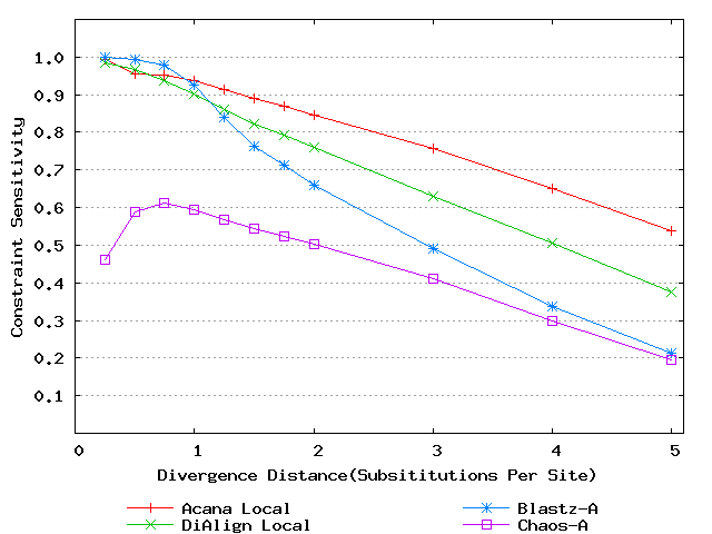
Figure 1: Comparison of constraint sensitivities and specificities of local alignment tools using benchmark DNA sequences, methods and results from Pollard et al. [2004]. Divergence distances in x-axis are measured by the number of substitutions per site in simulated sequences. The larger the number of substitutions per site, the larger the divergence distances. (a) Constraint sensitivities (b) Constraint specificities.
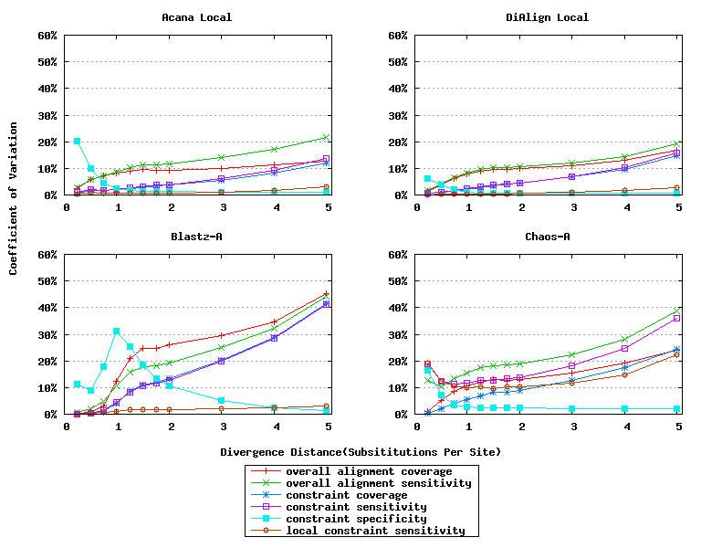
Figure 2: Coefficients of variation of local alignment tools. Divergence distances in x-axis are measured by the number of substitutions per site in simulated sequences. The larger the number of substitutions per site, the larger the divergence distances.
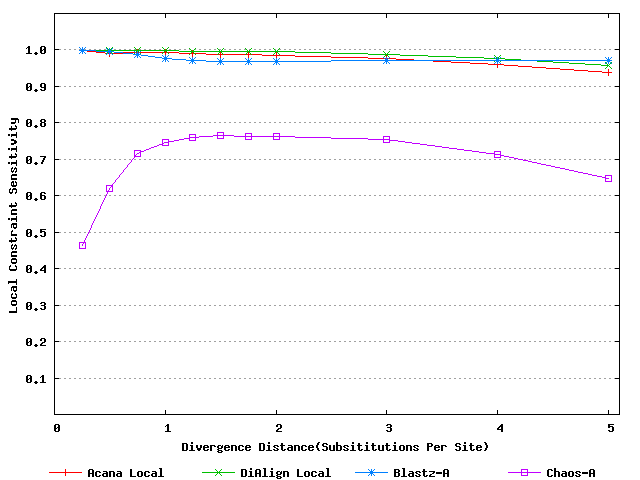
Figure 3: Local constraint sensitivities of local alignment tools. Divergence distances in x-axis are measured by the number of substitutions per site in simulated sequences. The larger the number of substitutions per site, the larger the divergence distances.
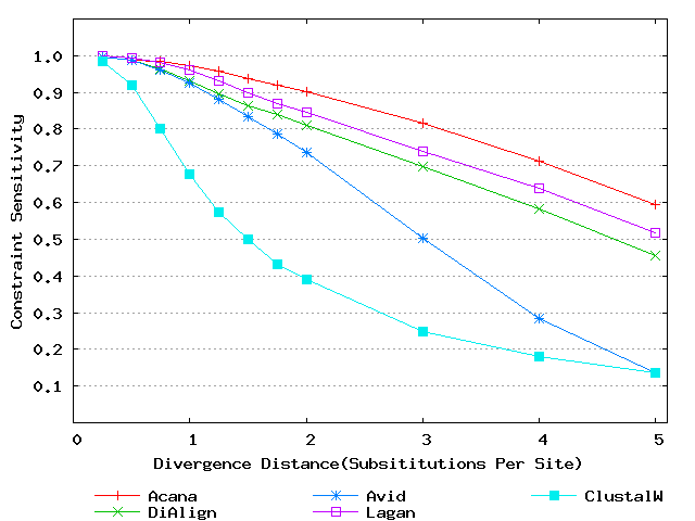
Figure 4: Comparison of constraint sensitivities and specificities of global alignment tools using benchmark DNA sequences, methods and results from Pollard et al. [2004]. Divergence distances in x-axis are measured by the number of substitutions per site in simulated sequences. The larger the number of substitutions per site, the larger the divergence distances. (a) Constraint sensitivities (b) Constraint specificities.
Figure 5: Overall alignment sensitivities of global alignment tools. Divergence distances in x-axis are measured by the number of substitutions per site in simulated sequences. The larger the number of substitutions per site, the larger the divergence distances.
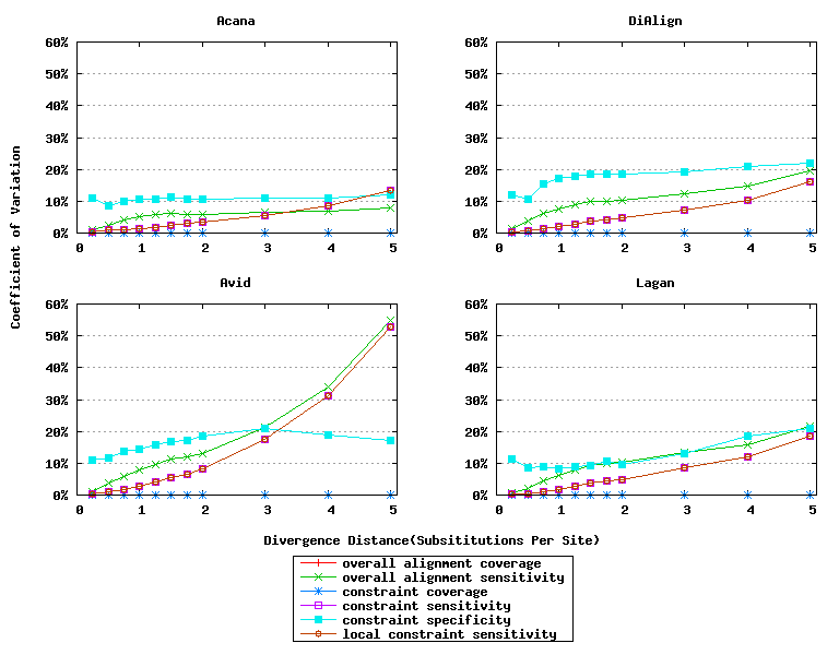
Figure 6: Coefficients of variation of global alignment tools. Divergence distances in x-axis are measured by the number of substitutions per site in simulated sequences. The larger the number of substitutions per site, the larger the divergence distances. For global alignment tools, the constraint sensitivity and local constraint sensitivity are equivalent (overlapped in plots), and both overall alignment coverage and constraint coverage are 1.0 over all divergence distances (no variation).
References
[Altschul and Gish 1996]
Altschul,S.F. and Gish,W. (1996) Local alignment statistics. Methods Enzymol., 266, 460-480.
[Brudno et al. 2003]
Brudno,M., Chapman,M., Göttgens,B., Batzoglou,S. and Morgenstern,B. (2003) Fast and sensitive multiple alignment of large genomic sequences. BMC Bioinformatics, 4, 66.
[Jurka 1998]
Jurka,J. (1998) Repeats in genomic DNA: mining and meaning. Curr Opin Struct Biol, 8, 333-337.
[Jurka 2000]
Jurka,J. (2000) Repbase update: a database and an electronic journal of repetitive elements. Trends Genet., 16, 418-420.
[Mayor et al. 2000]
Mayor,C., Brudno,M., Schwartz,J.R., Poliakov,A., Rubin,E.M., Frazer,K.A., Pachter,L.S. and Dubchak,I. (2000) VISTA : visualizing global DNA sequence alignments of arbitrary length. Bioinformatics, 16, 1046-1047.
[Morgenstern 1999]
Morgenstern,B. (1999) Dialign 2: improvement of the segment-to-segment approach to multiple sequence alignment. Bioinformatics, 15, 211-218.
[Morgenstern et al. 1996]
Morgenstern,B., Dress,A. and Werner,T. (1996) Multiple dna and protein sequence alignment based on segment-to-segment comparison. Proc. Natl. Acad. Sci. USA, 93, 12098-12103.
[Morgenstern et al. 1998]
Morgenstern,B., Frech,K., Dress,A. and Werner,T. (1998) Dialign: finding local similarities by multiple sequence alignment. Bioinformatics, 14, 290-294.
[Pollard et al. 2004]
Pollard,D.A., Bergman,C.M., Stoye,J., Celniker,S.E. and Eisen,M.B. (2004) Benchmarking tools for the alignment of functional noncoding DNA. BMC Bioinformatics, 5, 6.
[Schwartz et al. 2003]
Schwartz,S., Kent,W.J., Smit,A., Zhang,Z., Baertsch,R., Hardison,R.C., Haussler,D. and Miller,W. (2003) Human-mouse alignments with BLASTZ. Genome Res., 13, 103-107.
[Thompson et al. 1994]
Thompson,J.D., Higgins,D.G. and Gibson,T.J. (1994) Clustal w: improving the sensitivity of progressive multiple sequence alignment through sequence weighting, position-specific gap penalties and weight matrix choice. Nucleic Acids Res., 22, 4673-4680.