

Version 1.02
December 18, 2003
The GA/KNN selects the most discriminative variables for sample classification. It can be used for analysis of microarray gene expression data, proteomic data such as those from the SELDI-TOF, or other high-dimensional data. The current version provides four applications (see below).
1. To Get Started
On your unix or linux machine type: % gzip –dc ga_knn_1.01.tar.gz | tar –xvf –
to unpack the tar file. Individual source code files and example data files will appear.
% make
to compile. This should generate an executable “ga_knn”. The default compiler in the Makefile is gcc. If you have a C compiler, you need to change gcc to cc. See the Makefile for detail.
To run the program interactively% ./ga_knn arguments
‘.’ indicates that the ga_knn excutable is in the current directory.
To run the program in background% ./ga_knn arguments &
If you run the ga_knn by itself ./ga_knn, it will print out on screen all the arguments needed.
2. GA/KNN Arguments
-a application 1 = application 1 variable selection using all samples. 2 = application 2 variable selection using only the training samples. 3 = application 3 leave-one-out cross validation. 4 = application 4 split the data into training and test sets multiple times.
-c classification rule 1 = majority rule (default) 2 = consensus rule
-d chromosome length [integer] 10 or 20 should be ok for most cases.
-f data file name [char] if not in the same directory where the ga_knn is located, specify the full path, e.g., ~user/gaknn/data/data_file_name
-k k-nearest neighbors[integer] try 3 or 5 (depending on sample size and degree of heterogeneity in the data)
-n number of samples (specimens) in the data [integer]
-p print fitness score on screen for every generation of GA run 0 = no print 1 = print
-r target termination cutoff [integer] should be less or equal to the number of training samples
-s total number of solutions to be collected [integer] try 5000.
-t number of training samples [integer] should be less or equal to total number of samples.
-v number of variables (genes or m/z ratios) in your data [integer]
-N standardization, multiple choices are allowed e.g. -N 1 2
[default none] 1 = log2 transformation 2 = median centering of columns 3 = z-transformation of rows 4 = range scale (may be used for SELDI-TOF data)
Check the output file ga_knn_info.txt to see if correct arguments are used.
Examples:
./ga_knn –a 1 –c 1 –d 20 –f ExampleData.txt –k 3 –n 22 –r 19 –s 5000 –t 22 –v 3226 –N 1
Using utility 1, majority classification rule, chromosome length (d) 20, data file name ExampleData.txt, knn 3, total number of samples in the data 22, target termination criterion 19 (19 of the 22 samples need to be correctly classified), total number of solutions specified 5000, number of training samples 22 (all samples are used for selecting discriminative features), total number of variables (genes or m/z ratios) in the data 3226, standardization log2 transformation
./ga_knn –a 3 –c 1 –d 20 –f ExampleData.txt –k 3 –n 22 –r 19 –s 5000 –t 21 –v 3226 –N 1
Leave-one-out cross validation is used, number of training samples 21
3. Utilities of the Algorithm
The current version (1.02) has four applications. It allows a user 1) to select the discriminative variables (e.g., genes in microarray data or m/z ratios in SELDI-TOF proteomics data) using all samples; 2) to predict the classes of the test samples using the discriminative variables selected using the training set. The first t samples (the number following –t argument) will be taken as the training samples and the remaining as the test samples; 3) to perform a leave-one-out cross-validation (LOOCV); and 4) to assess the classification strength using multiple test sets of the same data.
Application 1 allows a user to select a subset of discriminative variables (features) using all samples. The variables are subsequently rank ordered according to the number of times it being selected. Three output files are generated for this application ga_knn_info.txt, selection_count.txt and variable_ranked_by_GA_KNN.txt. Descriptions of the output files can be found in 0readme.txt in the Example directory.
./ga_knn –a 1 –c 1 –d 20 –f ExampleData.txt –k 3 –n 22 –r 19 –s 5000 –t 22 –v 3226 –N 1
Note: the number of samples in training set is equal to the total number of samples.
Application 2 allows a user to specify a portion of the samples as the training samples for variable selection. The variables selected are subsequently used to predict the classes of the remaining (test set) samples. Many different numbers of top-ranked variables are used for the prediction, ranging from top 1 to 200 (if more than 200 variables are available). There are two more output files: prediction_test_set.txt and test_set_update.txt, in addition to the three listed in Application 1. Both files are updated every 500 near-optimal solutions. Again, descriptions of the output files can be found in 0readme.txt in the Example directory.
./ga_knn –a 2 –c 1 –d 20 –f ExampleData.txt –k 3 –n 22 –r 16 –s 5000 –t 17 –v 3226 –N 1
The difference between Applications 1 and 2 is that one uses all samples as training samples while the other uses a portion of it.
Application 3 allows a user to perform a leave-one-out cross-validation (LOOCV). Each of the samples is set aside and the remaining ones are used for variable selection. The variables selected are then used to predict the class of the one that is set aside. Many different numbers of top-ranked variables are used for the prediction. The two additional output files are loocv_update.txt and prediction_loocv.txt. Again, these files are updated every 500 near-optimal solutions.
./ga_knn –a 3 –c 1 –d 20 –f ExampleData.txt –k 3 –n 22 –r 19 –s 5000 –t 21 –v 3226 –N 1
Note: the number of training samples is one less than the total number of samples.
Application 4 allows a user to carry out multiple splits of the data set. For each split, the training samples are used for variable selection. The variables selected are subsequently used to predict the classes of the test samples. The default number of splits is 20. This can be changed by setting the numRuns in the main.c (line ~219) to the number desired (current: numRuns=20).
./ga_knn –a 4 –c 1 –d 20 –f ExampleData.txt –k 3 –n 22 –r 16 –s 5000 –t 17 –v 3226 –N 1
The difference between the Applications 2 and 4 is that in Application 2, the first 17 are used as the training sample whereas in Application 4, the training samples are randomly selected (without replacement). In addition, Application 2 only splits the data set once (the first 17 as training and remaining 5 as test samples). However, Application 4 randomly splits the data multiple times (default is 20) with a proportional number of samples in each class in both training and test sets.
Also, for a data set of this size, LOOCV instead of leave-many-out is as commended.
4. Input File Format
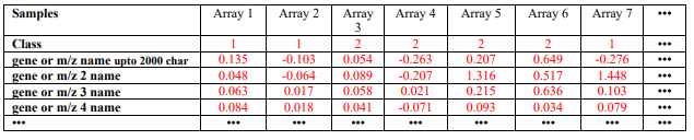
Only one data file is needed for the GA/KNN program. The current version of the GA/KNN algorithm only takes a tab delimited text file as the data file (containing both training and test samples). The file format is similar to that for Eisen’s clustering program, except that the second row of this file must contain class information for the samples (see Table 1 below for an example). For the test set samples, one may arbitrarily assign any class that is different from the classes of the training samples. For instance, the classes for the training samples are 0, 1 and 2, the test samples may be 9. However, to use application 4 to study the sensitivity and specificity of the algorithm, correct class types must be specified for both training and test samples. Make sure there are no empty tabs at the end of each line or extra empty line at the end of the file. These empty characters are not visible by eye, but will cause the program to stop. A class type 99 is used as default when a classification can not be made (each of the neighbors is a unique class and no majority votes).
KNN: For most of cases, k=3 or 5 should work well. However, if dye-swaps were used in the experiments, one should be careful. Since the dye effects could drive the separation. In other words, the KNN could discover the “subclasses” which are in effect due to the dye effects. In this case, one could increase the k to force all replicate hybs as one class. For instance, if 8 replicate hybs (4 labeled one way and 4 labeled the other way) were carried out for one treatment group and clearly there were dye effects, then, one should try a k of 5.
There are two classification rules (consensus and majority) in knn. A consensus rule implies that all k neighbors must agree whereas a majority rule means that most of the neighbors must agree when they make a vote. The default classification rule in GA/KNN is the majority rule, as recommended.
Chromosome length (d): In general, one could try a couple of choices to see if the results are sensitive. Without prior knowledge, I would chose a d in proportional to the number of samples. If the number of samples is small (e.g., under 10), one might use a d of 5 or 10. If the number of samples is between 10 and 20, I would use a d of 10, 15, or 20. For large data sets (> 30 samples), I would use a d of 20 or 30. My experience is that the ranks of variables are not very sensitive to the choice of d. A large d is computationally more intensive that a small d.
Termination cutoff: This is the fitness score cutoff to declare a near-optimal solution. This is the number of samples that must be correctly classified (based on the classification rule, see above KNN) in order to declare a near-optimal solution. When the fitness score is equal to or greater than the cutoff, the chromosome that gives the corresponding fitness score is saved. We refer to this chromosome as the near-optimal solution. It contains d variables (e.g., genes or m/z) indices. The search starts over with new sets of randomly initialized chromosomes. When many such near-optimal solutions have been obtained, the program ranks the variables according to the frequency of variable selection into these near-optimal solutions. The results are saved into two files selection_count.txt and variable_ranked_by_GA_KNN.txt. Those two files are updated every 500 near-optimal solutions.
Depending on the nature of the data, if the classes are quite different, one could set the termination fitness cutoff close to the number of samples, as seen in the above example. It should be a good idea not to require a perfect classification, even it is possible. This way the presence of potential outlier samples will have minimal effects on variable selection. When multiple classes exist, often, a nearperfect classification is not possible. In this case, one could do a test run by setting the last parameter in the parameter file to 1. This will allow the program to print out the fitness scores on screen as the search proceeds. Let it run for a couple of times (to stop the run: ctrl/C) and see what the fitness score it can reach around 10 to 20 generations. Then chose the fitness score around generations 10 as the termination fitness cutoff.
Number of near-optimal solutions: If the classes are quite different, a near-optimal solution should be found quickly (e.g., in less than 5 generations). This suggests that many subsets of variables that can discriminate between the classes of samples exist. One should let it run for a while (e.g., 5000 to 20000) to see if the ranks of the top variables stabilize. It is also possible that for some data sets a smaller number of solutions may be adequate. It is important to know that GA/KNN is a stochastic process; exact ranks order of the variables between runs may be not possible.
Contact

References
- Li L, Darden TA, Weinberg CR, Levine AJ, Pedersen LG. (2001) Gene assessment and sample classification for gene expression data using a genetic algorithm/k-nearest neighbor method. Comb. Chem. High Throughput Screen. 4, 727-739.
- Li L, Weinberg CR, Darden TA, and Pedersen LG. (2001) Gene selection for sample classification based on gene expression data: study of sensitivity to choice of parameters of the GA/KNN method. Bioinformatics, 17, 1131-1142.
- Li L, Umbach DM, Terry P, and Taylor JA. Application of the GA/KNN algorithm to SELDI proteomic data. Bioinformatics, in press.